Tutorials and Examples

Here, you can find detailed explanations on how to build and train specific models with GradValley.jl.

A LeNet-like model for handwritten digit recognition

In this tutorial, we will learn the basics of GradValley.jl while building a model for handwritten digit recognition, reaching approximately 99% accuracy on the MNIST-dataset. The whole code at once can be found here.

Importing modules

using GradValley # the master module of GradValley.jl
using GradValley.Layers # The "Layers" module provides all the building blocks for creating a model. 
using GradValley.Optimization # The "Optimization" module provides different loss functions and optimizers.

Using the dataset

We will use the MLDatasets package which downloads the MNIST-dataset for us automatically. If you haven't installed MLDatasets yet, write this for installation:

import Pkg; Pkg.add("MLDatasets")

Then we can import MLDatasets:

using MLDatasets # a package for downloading datasets

Splitting up the dataset into a train and a test partition

The MNIST-dataset contains 70,000 images, we will use 60,000 images for training the network and 10,000 images for evaluating accuracy.

# initialize train- and test-dataset
mnist_train = MNIST(:train) 
mnist_test = MNIST(:test)

Using GradValley.DataLoader for handling data

A typical workflow when dealing with datasets is to use the GradValley.DataLoader struct. A data loader makes it easy to iterate directly over the batches in a dataset. Due to better memory efficiency, the data loader loads the batches just in time. When initializing a data loader, we specify a function that returns exactly one element from the dataset at a given index. We also have to specify the size of the dataset (e.g. the number of images). All parameters that the data loader accepts (see Reference for more information):

DataLoader(get_function::Function, dataset_size::Integer; batch_size::Integer=1, shuffle::Bool=false, drop_last::Bool=false)

Now we write the get function for the two data loaders.

# function for getting an image and the corresponding target vector from the train or test partition
function get_element(index, partition)
    # load one image and the corresponding label
    if partition == "train"
        image, label = mnist_train[index]
    else # test partition
        image, label = mnist_test[index]
    end
    # add channel dimension and rescaling the values to their original 8 bit gray scale values
    image = reshape(image, 28, 28, 1) .* 255
    # generate the target vector from the label, one for the correct digit, zeros for the wrong digits
    # the element type of the image is Float32, so the target vector should have the same element type
    target = zeros(Float32, 10) 
    target[label + 1] = 1.f0

    return image, target
end

We can now initialize the data loaders.

# initialize the data loaders
train_data_loader = DataLoader(index -> get_element(index, "train"), length(mnist_train), batch_size=32, shuffle=true)
test_data_loader = DataLoader(index -> get_element(index, "test"), length(mnist_test), batch_size=32)

If you want to force the data loader to load the data all at once, you could do:

# force the data loaders to load all the data at once into memory, depending on the dataset's size, this may take a while
train_data = train_data_loader[begin:end]
test_data = test_data_loader[begin:end]

Building the neuronal network aka. the model

The recommend way to build feed forward models is to use the GradValley.Layers.SequentialContainer struct. A SequtialContainer can take an array of layers or other containers (sub-models). While forward-pass, the given inputs are sequentially propagated through every layer (or sub-model) and the output will be returned. For more details, see Reference. The LeNet5 model is one of the earliest convolutional neuronal networks (CNNs) reaching approximately 99% accuracy on the MNIST-dataset. The LeNet5 is built of two main parts, the feature extractor and the classifier. So it would be a good idea to clarify that in the code:

# Definition of a LeNet-like model consisting of a feature extractor and a classifier
feature_extractor = SequentialContainer([ # a convolution layer with 1 in channel, 6 out channels, a 5*5 kernel and a relu activation
                                         Conv(1, 6, (5, 5), activation_function="relu"),
                                         # an average pooling layer with a 2*2 filter (when not specified, stride is automatically set to kernel size)
                                         AvgPool((2, 2)),
                                         Conv(6, 16, (5, 5), activation_function="relu"),
                                         AvgPool((2, 2))])
flatten = Reshape((256, ))
classifier = SequentialContainer([ # a fully connected layer (also known as dense or linear) with 256 in features, 120 out features and a relu activation
                                  Fc(256, 120, activation_function="relu"),
                                  Fc(120, 84, activation_function="relu"),
                                  Fc(84, 10),
                                  # a softmax activation layer, the softmax will be calculated along the first dimension (the features dimension)
                                  Softmax(dims=1)])
# The final model consists of three different submodules, 
# which shows that a SequentialContainer can contain not only layers, but also other SequentialContainers
model = SequentialContainer([feature_extractor, flatten, classifier])

# After a model is initialized, its parameters are Float32 arrays by default. The input to the model must always be of the same element type as its parameters!
# You can change the device (CPU/GPU) and element type of the model's parameters with the function module_to_eltype_device!
# The element type of our data (image/target) is already Float32 and because this LeNet is such a small model, using the CPU is just fine.

Printing a nice looking summary of the model

Summarizing a model and counting the number of trainable parameters is easily done with the GradValley.Layers.summarie_model function.

# printing a nice looking summary of the model
summary, num_params = summarize_model(model)
println(summary)

Defining hyperparameters

Before we start to train and test the model, we define all necessary hyperparameters. If we want to change the learning rate or the loss function for example, this is the one place to do this.

# defining hyperparameters
loss_function = mse_loss # mean squared error
learning_rate = 0.05
optimizer = MSGD(model, learning_rate, momentum=0.5) # momentum stochastic gradient descent with a momentum of 0.5
epochs = 5 # 5 or 10, for example

Train and test the model

The next step is to write a function for training the model using the above defined hyperparameters. For example, the network is trained 5 or 10 times (epochs) with the entire training data set. After each batch, the weights/parameters of the network are adjusted/optimized. However, we want to test the model after each epoch, so we need to write a function for evaluating the model's accuracy first.

# evaluate the model's accuracy
function test()
    num_correct_preds = 0
    avg_test_loss = 0
    for (batch, (images_batch, targets_batch)) in enumerate(test_data_loader)
        # computing predictions
        predictions_batch = model(images_batch) # equivalent to forward(model, images_batch)
        # checking for each image in the batch individually if the prediction is correct
        batch_size = size(predictions_batch)[end] # the batch dimension is always the last dimension
        for index_batch in 1:batch_size
            single_prediction = predictions_batch[:, index_batch]
            single_target = targets_batch[:, index_batch]
            if argmax(single_prediction) == argmax(single_target)
                num_correct_preds += 1
            end
        end
        # adding the loss for measuring the average test loss
        avg_test_loss += loss_function(predictions_batch, targets_batch, return_derivative=false)
    end

    accuracy = num_correct_preds / size(test_data_loader) * 100 # size(data_loader) returns the dataset size
    avg_test_loss /= length(test_data_loader) # length(data_loader) returns the number of batches

    return accuracy, avg_test_loss
end

# train the model with the above defined hyperparameters
function train()
    for epoch in 1:epochs

        @time begin # for measuring time taken by one epoch

            avg_train_loss = 0.00
            # iterating over the whole data set
            for (batch, (images_batch, targets_batch)) in enumerate(train_data_loader)
                # computing predictions
                predictions_batch = model(images_batch) # equivalent to forward(model, images_batch)
                # backpropagation
                zero_gradients(model) # reset the gradients
                loss, derivative_loss = loss_function(predictions_batch, targets_batch)
                backward(model, derivative_loss) # compute the gradients
                # optimize the model's parameters
                step!(optimizer)
                # printing status
                if batch % 100 == 0
                    image_index = batch * train_data_loader.batch_size
                    data_set_size = size(train_data_loader)
                    println("Batch $batch, Image [$image_index/$data_set_size], Loss: $(round(loss, digits=5))")
                end
                # adding the loss for measuring the average train loss
                avg_train_loss += loss
            end

            avg_train_loss /= length(train_data_loader)
            accuracy, avg_test_loss = test()
            print("Results of epoch $epoch: Avg train loss: $(round(avg_train_loss, digits=5)), Avg test loss: $(round(avg_test_loss, digits=5)), Accuracy: $accuracy%, Time taken:")

        end

    end
end

Run the training and save the trained model afterwards

When the file is run as the main script, we want to actually call the train() function and save the final model afterwards. We will use the BSON.jl package for saving the model easily.

# when this file is run as the main script,
# then train() is run and the final model will be saved using a package called BSON.jl
import Pkg; Pkg.add("BSON")
using BSON: @save # a package for saving and loading julia objects as files
if abspath(PROGRAM_FILE) == @__FILE__
    train()
    file_name = "MNIST_with_LeNet5_model.bson"
    @save file_name model
    println("Saved trained model as $file_name")
end

Use the trained model

If you want to easily use the trained model, you firstly need to import the necessary modules from GradValley. Then you can use the @load macro of BSON to load the model object. Now you can let the model make a few individual predictions, for example. Use this code in in another file.

# load the model and make some individual predictions

using GradValley
using GradValley.Layers 
using GradValley.Optimization
using MLDatasets
using BSON: @load

# load the pre-trained model
@load "MNIST_with_LeNet5_model.bson" model

# make some individual predictions
mnist_test = MNIST(:test)
for i in 1:5
    random_index = rand(1:length(mnist_test))
    image, label = mnist_test[random_index]
    # remember to add batch and channel dimensions and to rescale the image as was done during training and testing
    image_batch = reshape(image, 28, 28, 1, 1) .* 255
    prediction = model(image_batch)
    predicted_label = argmax(prediction[:, 1]) - 1
    println("Predicted label: $predicted_label, Correct Label: $label")
end

Running the file with multiple threads

It is heavily recommended to run this file, and any other files using GradValley, with multiple threads. Using multiple threads can make training and calculating predictions much faster. To do this, use the -t option when running a julia script in terminal/PowerShell/command line/etc. If your CPU has 24 threads, for example, then run:

julia -t 24 ./MNIST_with_LeNet5.jl

The specified number of threads should match the number of threads your CPU provides.

Results

These were my results after 5 training epochs: Results of epoch 5: Avg train loss: 0.00239, Avg test loss: 0.00248, Accuracy: 98.36%, Time taken: 5.649449 seconds (20.96 M allocations: 13.025 GiB, 10.04% gc time) On my Ryzen 9 5900X CPU (using all 24 threads, slightly overclocked), one epoch took around ~6 seconds (no compilation time), so the whole training (5 epochs) took around ~30 seconds (no compilation time).

Generic ResNet (18/34/50/101/152) implementation

The same code can be also found here.

This example shows the ResNet implementation used by the pre-trained ResNets. The function ResBlock generates a standard residual block (with one residual/skipped connection) with optional downsampling. On the other hand, the function ResBottelneckBlock generates a bottleneck residual block (a variant of the residual block that utilises 1x1 convolutions to create a bottleneck) with optional downsampling. The residual connections can be easily implemented using the GraphContainer. GraphContainer allows differentiation for any computational graphs (not only sequential graphs for which the SequentialContainer is intended). The function ResNet constructs a generic ResNet. The functions ResNetXX use this function to create the individual models.

Note that this implementation is inspired by this article.

# import GradValley
using GradValley
using GradValley.Layers

# define a ResBlock (with optional downsampling) 
function ResBlock(in_channels::Int, out_channels::Int, downsample::Bool)
    # define modules
    if downsample
        shortcut = SequentialContainer([
            Conv(in_channels, out_channels, (1, 1), stride=(2, 2), use_bias=false),
            BatchNorm(out_channels)
        ])
        conv1 = Conv(in_channels, out_channels, (3, 3), stride=(2, 2), padding=(1, 1), use_bias=false)
    else
        shortcut = Identity()
        conv1 = Conv(in_channels, out_channels, (3, 3), padding=(1, 1), use_bias=false)
    end

    conv2 = Conv(out_channels, out_channels, (3, 3), padding=(1, 1), use_bias=false)
    bn1 = BatchNorm(out_channels, activation_function="relu")
    bn2 = BatchNorm(out_channels) # , activation_function="relu"

    relu = Identity(activation_function="relu")

    # define the forward pass with the residual/skipped connection
    function forward_pass(modules, input)
        # extract modules from modules vector (not necessary (therefore commented out) because the forward_pass function is defined in the ResBlock function (not somewhere "outside").)
        # shortcut, conv1, conv2, bn1, bn2, relu = modules
        # compute shortcut
        output_shortcut = forward(shortcut, input)
        # compute sequential part
        output = forward(bn1, forward(conv1, input))
        output = forward(bn2, forward(conv2, output))
        # residual/skipped connection
        output = forward(relu, output + output_shortcut) 
        
        return output
    end

    # initialize a container representing the ResBlock
    modules = [shortcut, conv1, conv2, bn1, bn2, relu]
    res_block = GraphContainer(forward_pass, modules)

    return res_block
end

# define a ResBottelneckBlock (with optional downsampling) 
function ResBottelneckBlock(in_channels::Int, out_channels::Int, downsample::Bool)
    # define modules
    shortcut = Identity()   

    if downsample || in_channels != out_channels
        if downsample
            shortcut = SequentialContainer([
                Conv(in_channels, out_channels, (1, 1), stride=(2, 2), use_bias=false),
                BatchNorm(out_channels)
            ])
        else
            shortcut = SequentialContainer([
                Conv(in_channels, out_channels, (1, 1), use_bias=false),
                BatchNorm(out_channels)
            ])
        end
    end

    conv1 = Conv(in_channels, out_channels ÷ 4, (1, 1), use_bias=false)
    if downsample
        conv2 = Conv(out_channels ÷ 4, out_channels ÷ 4, (3, 3), stride=(2, 2), padding=(1, 1), use_bias=false)
    else
        conv2 = Conv(out_channels ÷ 4, out_channels ÷ 4, (3, 3), padding=(1, 1), use_bias=false)
    end
    conv3 = Conv(out_channels ÷ 4, out_channels, (1, 1), use_bias=false)

    bn1 = BatchNorm(out_channels ÷ 4, activation_function="relu")
    bn2 = BatchNorm(out_channels ÷ 4, activation_function="relu")
    bn3 = BatchNorm(out_channels) # , activation_function="relu"

    relu = Identity(activation_function="relu")

    # define the forward pass with the residual/skipped connection
    function forward_pass(modules, input)
        # extract modules from modules vector (not necessary (therefore commented out) because the forward_pass function is defined in the ResBlock function (not somewhere "outside").)
        # shortcut, conv1, conv2, conv3, bn1, bn2, bn3, relu = modules
        # compute shortcut
        output_shortcut = forward(shortcut, input)
        # compute sequential part
        output = forward(bn1, forward(conv1, input))
        output = forward(bn2, forward(conv2, output))
        output = forward(bn3, forward(conv3, output))
        # residual/skipped connection
        output = forward(relu, output + output_shortcut) 
        
        return output
    end

    # initialize a container representing the ResBlock
    modules = [shortcut, conv1, conv2, conv3, bn1, bn2, bn3, relu]
    res_bottelneck_block = GraphContainer(forward_pass, modules)

    return res_bottelneck_block
end

# define a ResNet 
function ResNet(in_channels::Int, ResBlock::Union{Function, DataType}, repeat::Vector{Int}; use_bottelneck::Bool=false, classes::Int=1000)
    # define layer0
    layer0 = SequentialContainer([
        Conv(in_channels, 64, (7, 7), stride=(2, 2), padding=(3, 3), use_bias=false),
        BatchNorm(64, activation_function="relu"),
        MaxPool((3, 3), stride=(2, 2), padding=(1, 1))
    ])

    # define number of filters/channels
    if use_bottelneck
        filters = Int[64, 256, 512, 1024, 2048]
    else
        filters = Int[64, 64, 128, 256, 512]
    end

    # define the following modules
    layer1_modules = [ResBlock(filters[1], filters[2], false)]
    for i in 1:repeat[1] - 1
        push!(layer1_modules, ResBlock(filters[2], filters[2], false))
    end
    layer1 = SequentialContainer(layer1_modules)

    layer2_modules = [ResBlock(filters[2], filters[3], true)]
    for i in 1:repeat[2] - 1
        push!(layer2_modules, ResBlock(filters[3], filters[3], false))
    end
    layer2 = SequentialContainer(layer2_modules)

    layer3_modules = [ResBlock(filters[3], filters[4], true)]
    for i in 1:repeat[3] - 1
        push!(layer3_modules, ResBlock(filters[4], filters[4], false))
    end
    layer3 = SequentialContainer(layer3_modules)

    layer4_modules = [ResBlock(filters[4], filters[5], true)]
    for i in 1:repeat[4] - 1
        push!(layer4_modules, ResBlock(filters[5], filters[5], false))
    end
    layer4 = SequentialContainer(layer4_modules)

    gap = AdaptiveAvgPool((1, 1))
    flatten = Reshape((filters[5], ))
    fc = Fc(filters[5], classes)

    # initialize a container representing the ResNet
    res_net = SequentialContainer([layer0, layer1, layer2, layer3, layer4, gap, flatten, fc])

    return res_net
end

# construct a ResNet18
function ResNet18(in_channels=3, classes=1000)
    return ResNet(in_channels, ResBlock, [2, 2, 2, 2], use_bottelneck=false, classes=classes)
end

# construct a ResNet34
function ResNet34(in_channels=3, classes=1000)
    return ResNet(in_channels, ResBlock, [3, 4, 6, 3], use_bottelneck=false, classes=classes)
end

# construct a ResNet50
function ResNet50(in_channels=3, classes=1000)
    return ResNet(in_channels, ResBottelneckBlock, [3, 4, 6, 3], use_bottelneck=true, classes=classes)
end

# construct a ResNet101
function ResNet101(in_channels=3, classes=1000)
    return ResNet(in_channels, ResBottelneckBlock, [3, 4, 23, 3], use_bottelneck=true, classes=classes)
end

# construct a ResNet152
function ResNet152(in_channels=3, classes=1000)
    return ResNet(in_channels, ResBottelneckBlock, [3, 8, 36, 3], use_bottelneck=true, classes=classes)
end

It is heavily recommended to run this file (or the file in which you include and use ResNet.jl), and any other files using GradValley, with multiple threads. Using multiple threads can make training and calculating predictions much faster. To do this, use the -t option when running a julia script in terminal/PowerShell/command line/etc. If your CPU has 24 threads, for example, then run:

julia -t 24 ./ResNet.jl

The specified number of threads should match the number of threads your CPU provides.

Deep Convolutional Generative Adversarial Network (DCGAN) on CelebA-HQ

This example/tutorial can be seen as a reimplementation of PyTorch's DCGAN Tutorial with the difference that we are using CelebA-HQ (approx. 30,000 images) here instead of the normal CelebA (approx. 200,000 images) dataset. Note that this tutorial doesn't cover the theory behind DCGANs, it just focuses on the implementation in Julia with GradValley.jl. You can find detailed information about the theory and a step by step implementation in the awesome PyTorch DCGAN Tutorial.

The entire code, split into 5 files, can be found here.

Data preparation

Because loading and preprocessing 30,000 images takes some time, it would be a big waste of time to reload and prepare the dataset for each new training. Instead, we outsource the data preprocessing to another script and save the prepared data as a .jld2 file using FileIO.

We don't use CelebA-HQ because it's high quality. We could also just the use the normal version of CelebA, however, CelebA-HQ is a much smaller dataset and therefore easier to handle. I recommend to download the 256x256 version of CelebA-HQ because we only need 64x64 images for the DCGAN. Make sure all images are in a decompressed folder. This folder should contain 30,000 files.

The preprocessing of the images is done with the help of Images.jl and ImageTransformations.jl The included file preprocessing_for_resnets.jl is the file which is normally used by the pre-trained ResNets. It contains some useful utilities for preprocessing images. So it is useful for this DCGAN Tutorial as well. We will use GradValley's DataLoader to load the images into batches.

using GradValley
include("preprocessing_for_resnets.jl")
using FileIO

# make sure there is an / at the end of the data_directory string
data_directory = "F:/archive (1)/celeba_hq_256/" # replace the string with your path to the folder containing the images
files = readdir(data_directory)
dataset_size = length(files) # aka number of files/images

dtype = Float64 # Float64 is heavily recommended here, we can switch to Float32 for training any way
image_size = 64
batch_size = 128

# get function for the data loader that reads and transforms an image
function get_image(index::Integer)
    image = read_image_from_file(data_directory * files[index])
    image_size = 64
    # convert the image to the element type dtype and scale the values accordingly
    image = convert_image_eltype(image, dtype)
    # resize equivalent to torchvision's resize with one integer given as size argument
    width, height, channels = size(image)
    # print an error if the number of channels is not equal to 3 (rgb-images), important for normalization
    if channels != 3
        error("get_image: error while preprocessing, the image is expected to have 3 channels, however, $channels channel(s) was/were found")
    end
    # keeping the aspect ratio
    if height >= width
        new_size = (image_size, convert(Int, trunc(image_size * (height/width))), channels)
    elseif width > height
        new_size = (convert(Int, trunc(image_size * (width/height))), image_size, channels)
    end
    image = imresize(image, new_size)
    # desired size after cropping
    crop_size = (image_size, image_size)
    # center crop equivalent to torchvision's center crop 
    image = center_crop(image, crop_size[1], crop_size[2])
    # mean and standard deviation for normalization (separately for each channel)
    mean = [0.5, 0.5, 0.5]
    std = [0.5, 0.5, 0.5]
    # normalize equivalent to torchvision's normalize 
    image = normalize(image, mean, std)

    return (image, )
end

# initialize the data loader for loading the images into batches
dataloader = DataLoader(get_image, dataset_size, batch_size=batch_size, shuffle=true)
num_batches = dataloader.num_batches
file_name = "CelebA-HQ_preprocessed.jld2" # you can change the file name/path here as well
println("Number of batches: $num_batches")

# data is a vector containing the image batches
data = Vector{Array{dtype, 4}}(undef, num_batches)
# iterate over the data loader and add the batches to the data vector
for (batch_index, (images_batch, )) in enumerate(dataloader)
    println("[$batch_index/$num_batches]")
    data[batch_index] = images_batch
end
# the vector containing the batches is stored in file_name under the "data" key
save(file_name, Dict("data" => data))

Training

We will continue with the actual training script. The structure is strongly orientated towards the mentioned PyTorch DCGAN tutorial. Most of the comments in the code were also adopted from the PyTorch tutorial. At the beginning, the hyperparameters and the models are defined. Most code is needed for the relatively complex training loop in the function train. In the first step, the discriminator is trained with a batch of only real images. In the second step, the discriminator is trained again. This time, however, the discriminator is trained with only fake images which were generated by the generator model immediately before. In the final step, the generator is trained by backpropagating the generator loss through the discriminator and then through the generator model. The parameters of the discriminator model are updated after step two, the generator's parameters are updated after step three.

The script works for both GPU and CPU. However, having a GPU is required when you expect fast training. You can get some good results when training on the GPU on Float32 for approx. 25 epochs. On my RTX 3090, this took only 5 to 10 minutes. Training for more epochs (e.g. 75) can further improve results. If you use Float64 instead, you may can get good results after fewer epochs. GPUs are usually much faster on Float32, so using Float64 might only make sense if you train on the CPU. The CPU is also faster on Float32 than on Float64, but the speed difference is significantly smaller than on the GPU. If you only have a CPU, it might be worth it to train on Float64 with fewer epochs, for example only for 10 epochs with Float64 instead of 25 with Float32. A 10 epoch long training with Float32 took approx. 5 hours on my Ryzen 9 5900X (while some other tasks were active in the background).

using GradValley
using GradValley.Layers
using GradValley.Optimization
using CUDA
using FileIO

# Load the preprocessed data
batches = load("CelebA-HQ_preprocessed.jld2", "data")

# Number of channels in the training images. For color images this is 3
nc = 3

# Size of z latent vector (i.e. size of generator input)
nz = 100

# Size of feature maps in generator
ngf = 64

# Size of feature maps in discriminator
ndf = 64

# Number of training epochs
# e.g. 25 epochs on Float32 for both GPU and CPU or 10 epochs on Float64 for the CPU
# if you have a good GPU, you can also try more epochs, for example with 75
num_epochs = 25

# Learning rate for optimizers
lr = 0.0002

# Beta1 hyperparameter for Adam optimizers
beta1 = 0.5

# eltype of data and parameters
# Float32 or Float64
dtype = Float32

generator = SequentialContainer([
    # input is Z, going into a convolution
    ConvTranspose(nz, ngf * 8, (4, 4), stride=(1, 1), padding=(0, 0), use_bias=false),
    BatchNorm(ngf * 8, activation_function="relu"),
    # state size. (ngf*8) x 4 x 4
    ConvTranspose(ngf * 8, ngf * 4, (4, 4), stride=(2, 2), padding=(1, 1), use_bias=false),
    BatchNorm(ngf * 4, activation_function="relu"),
    # state size. (ngf*4) x 8 x 8
    ConvTranspose(ngf * 4, ngf * 2, (4, 4), stride=(2, 2), padding=(1, 1), use_bias=false),
    BatchNorm(ngf * 2, activation_function="relu"),
    # state size. (ngf*2) x 16 x 16
    ConvTranspose(ngf * 2, ngf, (4, 4), stride=(2, 2), padding=(1, 1), use_bias=false),
    BatchNorm(ngf, activation_function="relu"),
    # state size. (ngf) x 32 x 32
    ConvTranspose(ngf, nc, (4, 4), stride=(2, 2), padding=(1, 1), use_bias=false, activation_function="tanh")
    # state size. (nc) x 64 x 64
])

discriminator = SequentialContainer([
    # input is (nc) x 64 x 64
    Conv(nc, ndf, (4, 4), stride=(2, 2), padding=(1, 1), use_bias=false, activation_function="leaky_relu:0.2"),
    # state size. (ndf) x 32 x 32
    Conv(ndf, ndf * 2, (4, 4), stride=(2, 2), padding=(1, 1), use_bias=false),
    BatchNorm(ndf * 2, activation_function="leaky_relu:0.2"),
    # state size. (ndf*2) x 16 x 16
    Conv(ndf * 2, ndf * 4, (4, 4), stride=(2, 2), padding=(1, 1), use_bias=false),
    BatchNorm(ndf * 4, activation_function="leaky_relu:0.2"),
    # state size. (ndf*4) x 8 x 8
    Conv(ndf * 4, ndf * 8, (4, 4), stride=(2, 2), padding=(1, 1), use_bias=false),
    BatchNorm(ndf * 8, activation_function="leaky_relu:0.2"),
    # state size. (ndf*8) x 4 x 4
    Conv(ndf * 8, 1, (4, 4), stride=(1, 1), padding=(0, 0), use_bias=false, activation_function="sigmoid")
])

# check if CUDA is available
use_cuda = CUDA.functional()
# move the model to the correct device and convert its parameters to the specified dtype
if use_cuda
    println("The GPU is used")
    module_to_eltype_device!(generator, element_type=dtype, device="gpu")
    module_to_eltype_device!(discriminator, element_type=dtype, device="gpu")
else
    println("The CPU is used")
    module_to_eltype_device!(generator, element_type=dtype, device="cpu")
    module_to_eltype_device!(discriminator, element_type=dtype, device="cpu")
end

# Setup the loss function
criterion = bce_loss

# Create batch of latent vectors that we will use to visualize the progression of the generator
if use_cuda
    fixed_noise = CUDA.randn(dtype, 1, 1, nz, 64)
else
    fixed_noise = randn(dtype, 1, 1, nz, 64)
end 

# Establish convention for real and fake labels during training
real_label = dtype(1)
fake_label = dtype(0)

# Setup Adam optimizers for both G and D
optimizerD = Adam(discriminator, learning_rate=lr, beta1=beta1, beta2=0.999)
optimizerG = Adam(generator, learning_rate=lr, beta1=beta1, beta2=0.999)

function train()
    # Training Loop

    # Lists to keep track of progress
    img_list = []
    G_losses = []
    D_losses = []
    global iters = 0

    println("Starting Training Loop...")
    # For each epoch
    for epoch in 1:num_epochs

        # save some interim results when using the CPU
        if !use_cuda && epoch == 6
            file_name_img_list = "img_list_intermediate_result.jld2"
            save(file_name_img_list, Dict("img_list" => img_list))
        end

        # For each batch in the data
        for (i, batch) in enumerate(batches)

            ############################
            # (1) Update D network: maximize log(D(x)) + log(1 - D(G(z)))
            ###########################
            ## Train with all-real batch
            zero_gradients(discriminator)

            if eltype(batch) != dtype
                batch = convert(Array{dtype, 4}, batch)
            end

            # Format batch
            if use_cuda
                real = CuArray(batch)
            else
                real = batch
            end

            b_size = size(real)[end]
            if use_cuda
                label = CUDA.fill(real_label, (1, 1, 1, b_size))
            else
                label = fill(real_label, (1, 1, 1, b_size))
            end
            # Forward pass real batch through D
            output = forward(discriminator, real)
            # Calculate loss on all-real batch
            errD_real, errD_real_derivative = criterion(output, label)
            # Calculate gradients for D in backward pass
            backward(discriminator, errD_real_derivative)
            D_x = sum(output) / length(output)

            ## Train with all-fake batch
            # Generate batch of latent vectors
            if use_cuda
                noise = CUDA.randn(dtype, 1, 1, nz, b_size)
            else
                noise = randn(dtype, 1, 1, nz, b_size)
            end
            # Generate fake image batch with G
            fake = forward(generator, noise)
            if use_cuda
                CUDA.fill!(label, fake_label)
            else
                fill!(label, fake_label)
            end
            # Classify all fake batch with D
            output = forward(discriminator, fake)
            # Calculate D's loss on the all-fake batch
            errD_fake, errD_fake_derivative = criterion(output, label)
            # Calculate the gradients for this batch, accumulated (summed) with previous gradients
            backward(discriminator, errD_fake_derivative)
            D_G_z1 = sum(output) / length(output)
            # Compute error of D as sum over the fake and the real batches
            errD = errD_real + errD_fake
            # Update D
            step!(optimizerD)

            ############################
            # (2) Update G network: maximize log(D(G(z)))
            ###########################
            zero_gradients(generator)
            # fake labels are real for generator cost
            if use_cuda
                CUDA.fill!(label, real_label) 
            else
                fill!(label, real_label) 
            end
            # Since we just updated D, perform another forward pass of all-fake batch through D
            output = forward(discriminator, fake)
            # Calculate G's loss based on this output
            errG, errG_derivative = criterion(output, label)
            # Calculate gradients for G
            # The gradient flow does not reach the generator automatically, 
            # so we have to do that manually by passing the gradient returned from the backward pass of the discriminator as the derivative_loss input to the generator backward call
            input_gradient = backward(discriminator, errG_derivative)
            backward(generator, input_gradient)
            D_G_z2 = sum(output) / length(output)
            # Update G
            step!(optimizerG)

            # Output training stats
            if i % 1 == 0 # i % 50 == 0
                println("[$epoch/$num_epochs][$i/$(235)]\tLoss_D: $(round(errD, digits=4))\tLoss_G: $(round(errG, digits=4))\tD(x): $(round(D_x, digits=4))\tD(G(z)): $(round(D_G_z1, digits=4)) / $(round(D_G_z2, digits=4))")
            end

            # Save Losses for potential plotting later
            push!(G_losses, errG)
            push!(D_losses, errD)

            # Check how the generator is doing by saving G's output on fixed_noise
            if (iters % 50 == 0) || ((epoch == num_epochs) && (i == length(batches)))
                # testmode!(generator)
                fake = forward(generator, fixed_noise)
                # trainmode!(generator)
                push!(img_list, fake)
            end

            global iters += 1
        end
    end

    return img_list, G_losses, D_losses
end

# Start training 
if use_cuda
    img_list, G_losses, D_losses = CUDA.@time train()
else
    img_list, G_losses, D_losses = @time train()
end

# move the intermediate results on fixed_noise in img_list and the models back to the CPU for saving
if use_cuda
    for i in eachindex(img_list)
        img_list[i] = convert(Array{dtype, 4}, img_list[i])
    end
    # note that clean_model_from_backward_information! runs automatically in the background when calling module_to_eltype_device! on a container
    module_to_eltype_device!(discriminator, element_type=dtype, device="cpu")
    module_to_eltype_device!(generator, element_type=dtype, device="cpu")
end

# Save the models 
file_nameD = "discriminator.jld2"
save(file_nameD, Dict("discriminator" => discriminator))
file_nameG = "generator.jld2"
save(file_nameG, Dict("generator" => generator))
# Save the image list (intermediate results on fixed_noise)
file_name_img_list = "img_list.jld2"
save(file_name_img_list, Dict("img_list" => img_list))

It is heavily recommended to run this file, and any other files using GradValley, with multiple threads. Using multiple threads can make training and calculating predictions on the CPU much faster. To do this, use the -t option when running a julia script in terminal/PowerShell/command line/etc. If your CPU has 24 threads, for example, then run:

julia -t 24 ./DCGAN.jl

The specified number of threads should match the number of threads your CPU provides.

Check results and run inference

The following script visualizes the intermediate outputs on fixed_noise by arranging them in a grid. To prevent the plot windows from closing immediately, readline is used to wait until enter is pressed in the console before displaying a new batch. The packages Plots.jl and Measures.jl are used for plotting.

using Plots, Measures, Images, FileIO

# plot all batches in img_list by arranging the images in a batch in a grid
# press enter in the console to continue
function show_img_list(img_list)
    for (i, img_batch) in enumerate(img_list)
        batch_size = size(img_batch)[end]

        image_plots = []
        for index_batch in 1:batch_size
            image = @view img_batch[:, :, :, index_batch]
            image = PermutedDimsArray(image, (3, 2, 1))

            # normalize
            min = minimum(image)
            max = maximum(image)
            norm(x) = (x - min) / (max - min)
            image = norm.(image)

            image = colorview(RGB, image)
            image_plot = plot(image)
            push!(image_plots, image_plot)
        end 

        # create a plot and display a gui window with the plot
        p = plot(image_plots..., framestyle=:none, border=:none, leg=false, ticks=nothing, margin=-1.5mm, left_margin=-1mm, right_margin=-1mm) # , show=true
        display(p)
        # prevent the window from closing immediately
        readline()
        # save the plot as an image file 
        savefig(p, "img_list_grid_$i.png")

        println("[$i/$(length(img_list))]")
    end
end

file_name_img_list = "img_list.jld2"
img_list = load(file_name_img_list, "img_list")
println(length(img_list))
img_list = img_list[end-9:end] # show only the last 10 batches
show_img_list(img_list)

The following script loads the generator model and generates some new images and saves them as independent image files.

using GradValley
using GradValley.Layers
using Images

num_images = 50
name_prefix = "fake"
format = ".jpeg"
# make sure there is an / at the end of the dist string
dist = "inference/"
!isdir(dist) && mkdir(dist)

# Size of z latent vector (i.e. size of generator input)
nz = 100

# Float32 or Float64
dtype = Float32

# convert a tensor of size (width, height, channels) to a 2d RGB image array
function tensor_to_image(tensor::AbstractArray{T, 3}) where T <: Real
    image = PermutedDimsArray(tensor, (3, 2, 1))
    image = colorview(RGB, image)
    return image
end

file_nameG = "generator.jld2"
generator = load(file_nameG, "generator")
# testmode!(generator)
module_to_eltype_device!(generator, element_type=dtype, device="cpu")

noise = randn(dtype, 1, 1, nz, num_images)
fake = generator(noise)
fake = @time generator(noise)

for i in 1:num_images
    image = @view fake[:, :, :, i]

    # normalize
    min = minimum(image)
    max = maximum(image)
    norm(x) = (x - min) / (max - min)
    image = norm.(image)

    image = tensor_to_image(image)

    file_path = dist * name_prefix * string(i) * format
    save(file_path, image)
end

Results

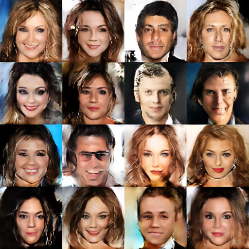
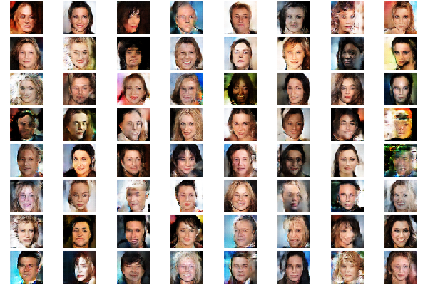
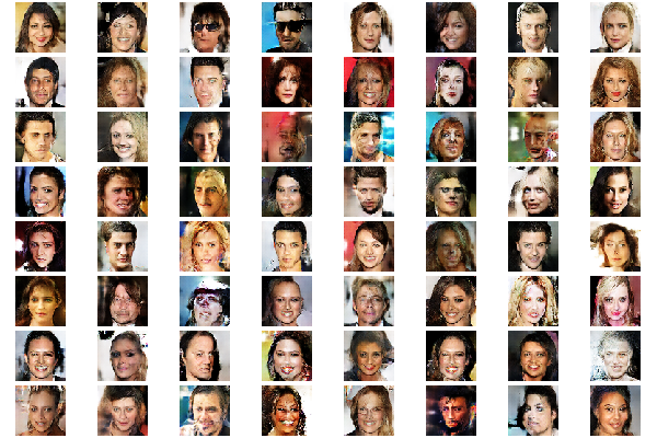
These are some example results after 25 and after 75 epochs of training on Float32:

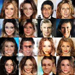
Bonus: I used this tool for upscaling the first image grid. After upscaling 2 times, I got the following result. The used image upscaler tool works with AI too, so please note that the upscaler can add details to the image that weren't there before.